Version Progression
Architecture (v2/v3 with BatchNorm)
Green = BatchNorm added in v2 (normalizes activations per-channel per-batch)
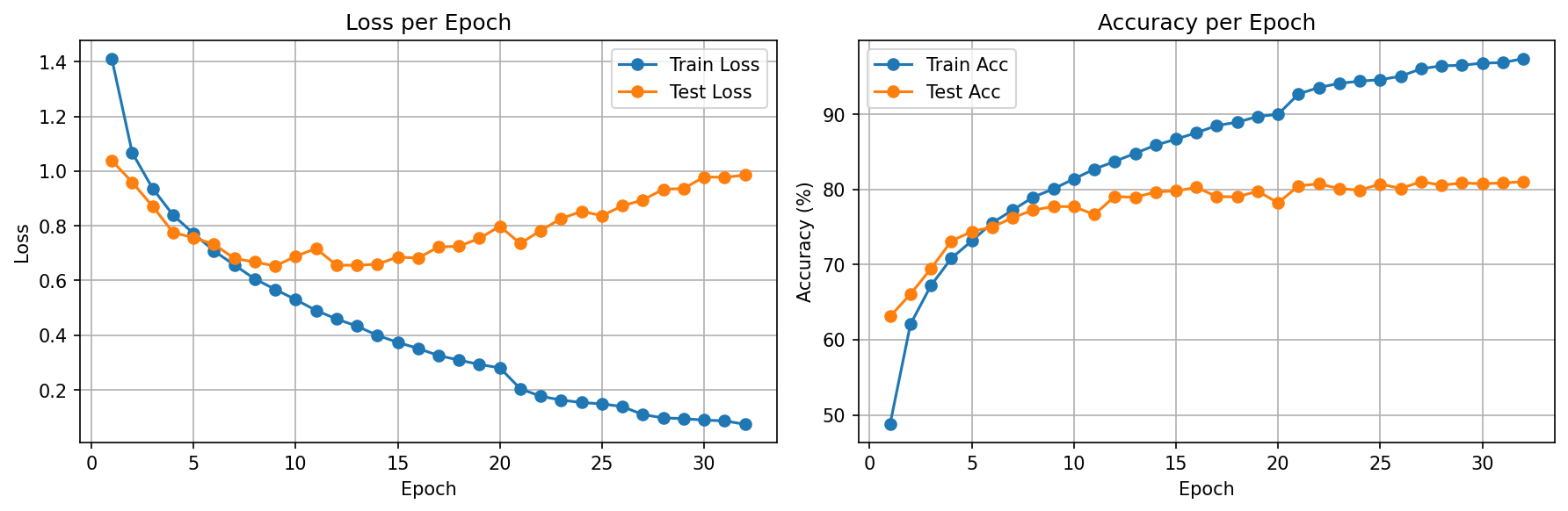
v3 Learning Rate Schedule
| Epoch Range | Learning Rate | Effect |
|---|---|---|
| 1 – 19 | 0.001000 | Initial training phase |
| 20 – 25 | 0.000500 | 1st reduction — +0.48% accuracy gain |
| 26 – 30 | 0.000250 | 2nd reduction — +0.28% gain |
| 31 – 32 | 0.000125 | 3rd reduction — no further gain, early stop |
Each halving yields less improvement — a clear sign the architecture itself is the bottleneck, not the optimizer.
Training Results
v1 — Baseline
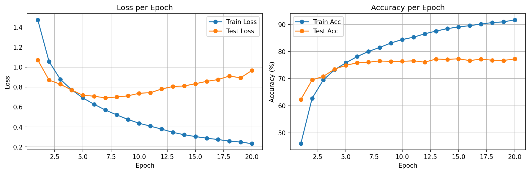
v2 — BatchNorm
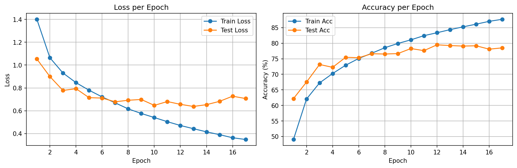
v3 — LR Scheduler
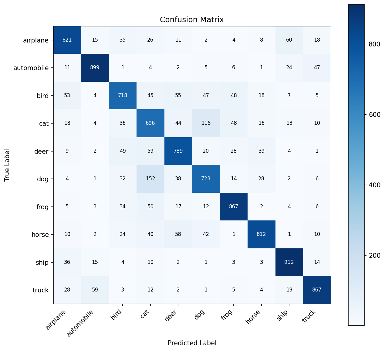
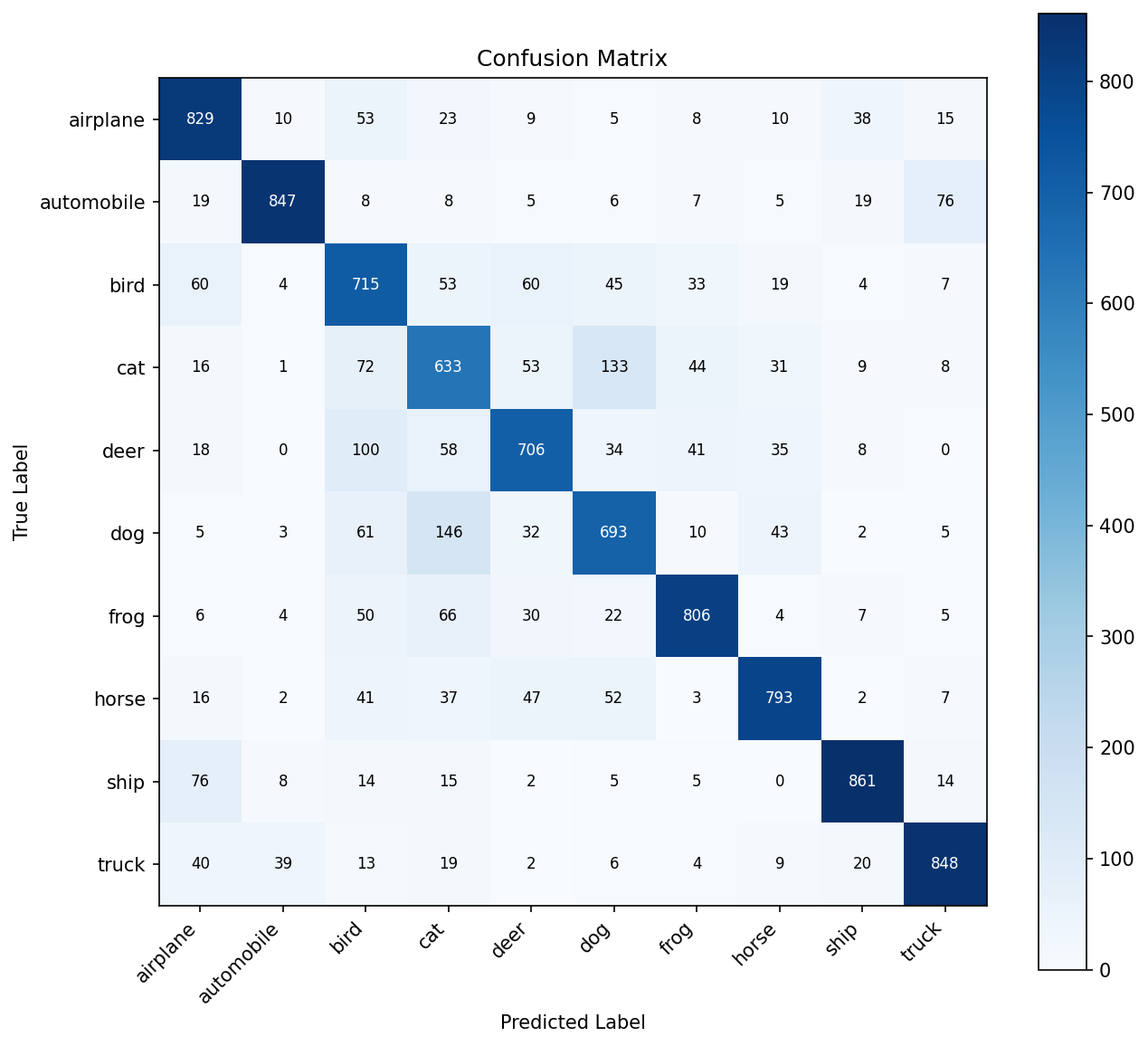
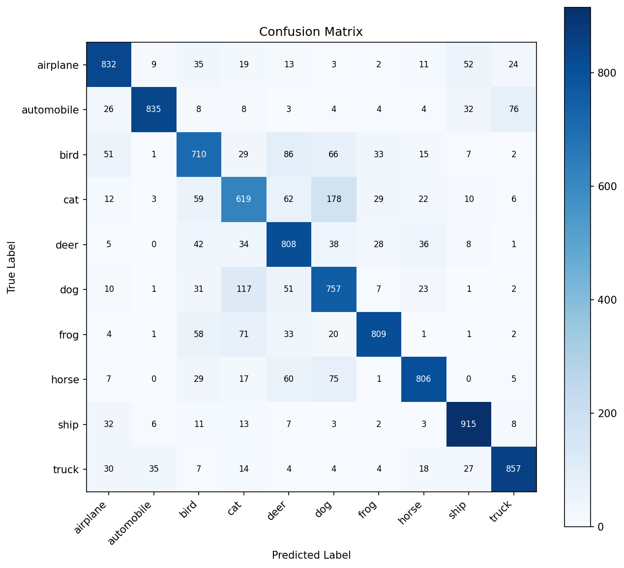
Hardest Class Pairs (Consistent Across All Versions)
These confusions are inherent to 32×32 resolution — even humans struggle. Higher resolution + pretrained features solve this.
Concepts Study Guide
Batch Normalization (BatchNorm)
BatchNorm normalizes the outputs of a layer across the current mini-batch to have mean=0 and variance=1. Then it applies two learnable parameters (γ and β) that let the network undo the normalization if it's not helpful. This combats internal covariate shift — the problem where each layer's input distribution keeps changing as earlier layers update.
Imagine a relay race where each runner expects the baton at a certain height. If runner 1 randomly changes their handoff height each lap, runner 2 wastes energy adapting. BatchNorm forces every handoff to happen at a standardized height, so each runner (layer) can focus on their own technique instead of constantly adjusting to unpredictable inputs.
μ_c = mean of all activations in channel c across the batch
σ_c = std of all activations in channel c across the batch
x_norm = (x - μ_c) / √(σ_c² + ε)
output = γ * x_norm + β (γ, β are learnable)
Training vs Evaluation: During training, it uses batch statistics. During evaluation, it uses running averages computed over the entire training set. This is another reason model.eval() matters.
Adding BatchNorm to v2 (Conv→BN→ReLU→Pool) boosted accuracy from 77.31% to 79.48% while halving the overfitting gap (15%→8%). It's the single most impactful regularization technique we've used — more effective than Dropout for conv layers.
Learning Rate Scheduling (ReduceLROnPlateau)
A fixed learning rate is a compromise: too large and training overshoots minima; too small and training is slow. ReduceLROnPlateau starts with a larger LR for fast initial progress, then automatically reduces it by a factor when the monitored metric stops improving for patience epochs.
Imagine pouring water into a cup. At first, you pour quickly to fill it fast (large LR). As it nears the top, you slow the pour to avoid spilling (smaller LR). ReduceLROnPlateau is like a sensor that says "the cup hasn't gotten fuller in 3 seconds, slow down the pour by half."
mode='max', # monitoring accuracy (higher is better)
factor=0.5, # multiply LR by 0.5 when triggered
patience=3 # wait 3 epochs of no improvement
)
0.001 → 0.0005 → 0.00025 → 0.000125 (each halving)
Key insight: The scheduler doesn't just "optimize better" — it rescues models from premature early stopping. Without it, v2 stopped at epoch 17. With it, v3 trained to epoch 32 because each LR reduction opened a new valley to explore.
v3 used ReduceLROnPlateau to squeeze +1.56% more accuracy beyond BatchNorm. But diminishing returns per reduction (0.48%→0.28%→0%) proved the architecture itself was the bottleneck, not the optimizer settings.
Overfitting vs Underfitting
Overfitting: The model memorizes training data patterns (including noise) but fails on new data. Symptom: high train accuracy, much lower test accuracy.
Underfitting: The model is too simple to capture the real patterns. Symptom: both train and test accuracy are low.
Overfitting is like a student who memorizes every practice exam word-for-word but can't answer rephrased questions. Underfitting is like a student who only skimmed the textbook — they can't answer any questions well. The sweet spot is understanding the concepts behind the examples.
v2: Train 87% / Test 79% → 8% gap = moderate (BN helped)
v3: Train 97% / Test 81% → 16% gap = overfitting returned
But v3 has the HIGHEST test accuracy — overfitting gap alone
doesn't tell you which model is best. The absolute test metric does.
Tools to fight overfitting: Dropout, BatchNorm, data augmentation, early stopping, weight decay, more training data, simpler model.
The v1→v2→v3 progression is a masterclass in the overfitting/accuracy tradeoff. v2's BatchNorm reduced the gap but v3's scheduler increased it — yet v3 was still the best model by test accuracy. The lesson: watch the absolute test metric, not just the gap.
Data Augmentation
Data augmentation applies random transformations (flips, crops, rotations, color jitter) to training images on-the-fly. Each epoch, the model sees slightly different versions of the same images. This acts as a regularizer — the model can't memorize specific pixel patterns.
Imagine learning to recognize your friend's face. You've only seen 100 photos. Data augmentation is like seeing those same photos in different lighting, from slightly different angles, sometimes flipped — suddenly your 100 photos feel like 1,000, and you recognize them in any condition.
transforms.RandomHorizontalFlip(), # 50% chance to mirror
transforms.RandomCrop(32, padding=4), # shift up to 4px
transforms.ToTensor(),
transforms.Normalize(mean, std)
])
Note: augmentation is ONLY applied to training data, never test/val
CIFAR-10 has only 50K training images of 32×32 pixels — much harder than MNIST. RandomHorizontalFlip and RandomCrop help the model generalize without needing more data. These same augmentations carry forward to every future project.
The "Scratch CNN Ceiling"
A shallow network (2-3 conv layers) can only learn low-to-mid-level features: edges, corners, simple textures. Distinguishing a cat from a dog requires high-level semantic features (ear shape, fur patterns, body posture) that need many more layers to build up.
Imagine describing the Mona Lisa. With 3 words, you might say "woman, dark, painting." With 30 words, you can describe her pose, expression, background. With 300 words, you capture subtleties. A 3-layer CNN is limited to "3-word descriptions" of images — enough for digits (simple shapes), not enough for cats vs dogs (complex objects).
CIFAR-10 (3 channels, 10 complex classes): 81% with 3 conv layers ✘
CIFAR-10 with ResNet-18 (18 layers): 93-95% ✔
Depth matters more than width for complex visual recognition.
This entire project exists to experience the ceiling. We tried every trick (BatchNorm, scheduling) and still couldn't break 81%. This makes the motivation for transfer learning visceral, not theoretical. You don't just read "deeper networks work better" — you prove it.
Lessons Learned
What's Next
The ceiling is clear: ~81% on CIFAR-10 with a scratch CNN. The next project uses Transfer Learning (ResNet18) on a harder task (100 sports classes) to show how pretrained features shatter this ceiling: 91% with feature extraction alone, 96-98% with fine-tuning.