Model Architecture
SimpleCNN
Training Configuration
| Parameter | Value | Why |
|---|---|---|
| Optimizer | Adam (lr=0.001) | Faster convergence than SGD for this simple task |
| Loss | CrossEntropyLoss | Standard for multi-class classification |
| Batch Size | 64 | Good balance of speed and gradient stability |
| Dropout | 0.5 on FC layer | Prevents overfitting; without it, train acc diverges from test |
| Early Stopping | patience=3 | Stopped at epoch 13; best checkpoint at epoch 10 |
| Data Split | 60K train / 10K test | Standard MNIST split; large test set is reliable |
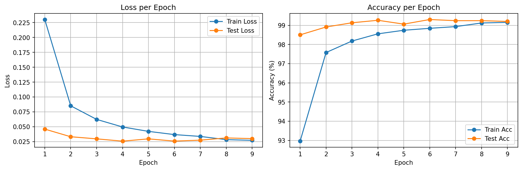
Training Results
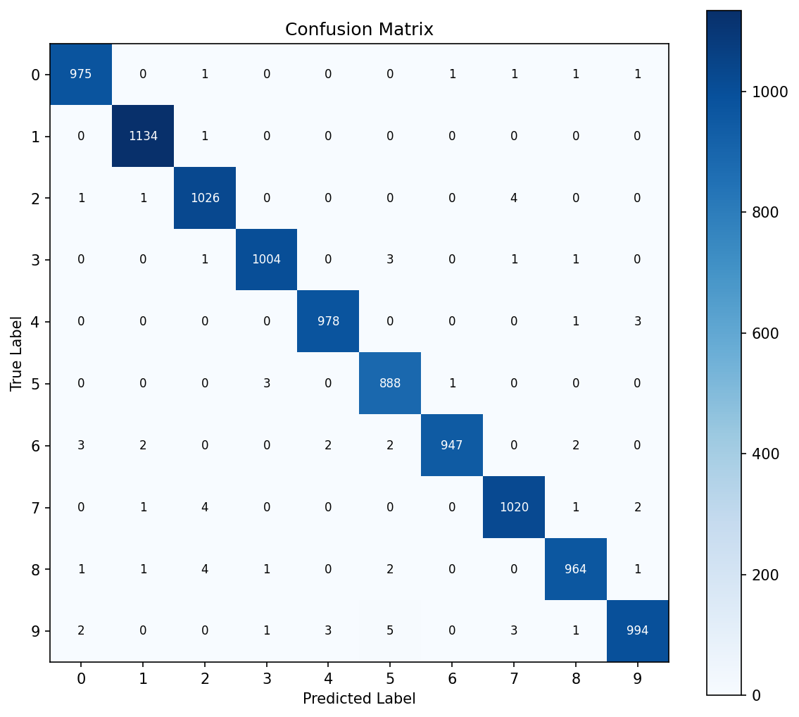
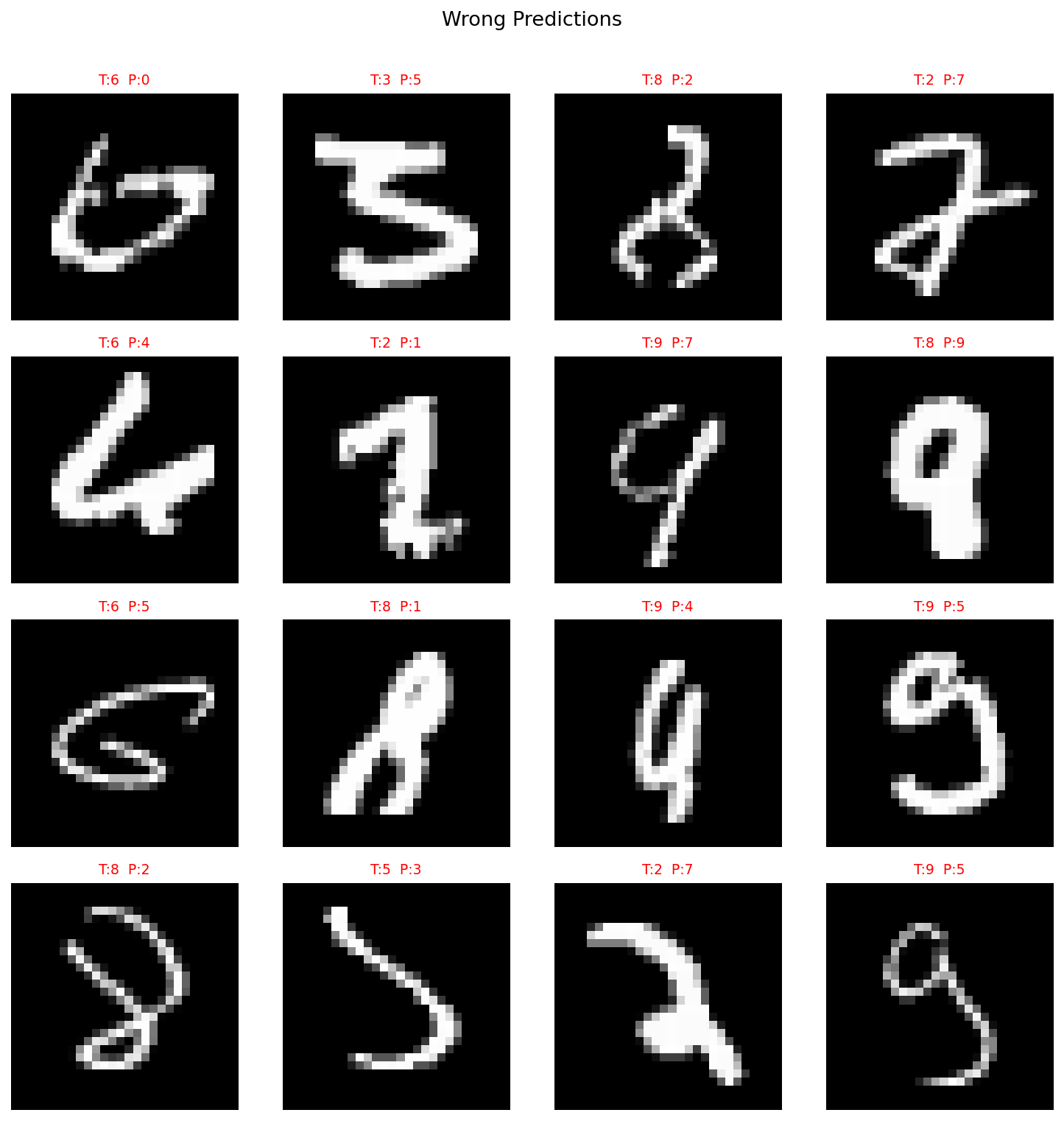
Hardest Digit Pairs
Concepts Study Guide
Convolution (Conv2d)
A convolution slides a small filter (kernel) across the input image, computing a dot product at each position. Each filter learns to detect a specific pattern — edges, corners, textures, etc.
Imagine reading a page with a magnifying glass. You scan a small area at a time (the kernel), looking for specific patterns. One magnifying glass might highlight vertical lines, another might highlight curves. Together, dozens of these "magnifying glasses" (filters) capture everything on the page.
Key parameters:
• in_channels / out_channels — how many input feature maps go in, how many filters (output maps) come out.
• kernel_size — the size of the sliding window (3×3 is most common).
• padding — adding zeros around the border so the output keeps the same spatial size.
Example: (28 + 2×1 - 3) / 1 + 1 = 28 → same size with padding=1
Conv layers are the backbone of any CNN. Our 2 conv layers extract increasingly abstract features: layer 1 finds edges, layer 2 combines edges into digit shapes.
ReLU (Rectified Linear Unit)
ReLU applies f(x) = max(0, x) element-wise. Without a nonlinear activation, stacking multiple linear layers would collapse into a single linear transformation — the network couldn't learn complex patterns.
Think of a neuron that only "fires" when excited. If the signal is positive (interesting pattern detected), pass it through. If negative (not relevant), shut it off completely. This simple on/off behavior, when combined across thousands of neurons, creates powerful pattern recognition.
ReLU(-3) = 0 | ReLU(0) = 0 | ReLU(5) = 5
ReLU is applied after every Conv layer and the first FC layer. It's the industry default because it's fast, simple, and avoids the vanishing gradient problem that plagues sigmoid/tanh in deep networks.
MaxPooling
MaxPool2d(2) slides a 2×2 window across the feature map and keeps only the maximum value. This halves the spatial dimensions (H and W), reducing computation and making the model invariant to small translations.
Imagine you divided a photo into 2×2 pixel blocks. From each block, you only keep the brightest pixel. You lose fine detail but keep the important structure — and the image is now 1/4 the size. This is exactly what MaxPooling does to feature maps.
Spatial dims halved: 28/2 = 14. Channels unchanged.
After each Conv+ReLU, we pool to shrink the feature map. This creates a hierarchy: early layers see fine details (14×14), later layers see abstract patterns (7×7). It also adds translation invariance — a digit shifted by 1 pixel still activates the same pooled region.
Dropout
During training, Dropout(p=0.5) randomly sets 50% of neuron outputs to zero each forward pass. This forces the network to not rely on any single neuron, building redundancy. During evaluation, all neurons are active (scaled to compensate).
Imagine a team where half the members randomly call in sick each day. The team learns to be resilient — no single person becomes a bottleneck, and everyone develops broader skills. On the day of the final presentation (evaluation), everyone shows up and the team performs at its best.
Evaluation: use all activations, multiply by (1-p) to compensate
model.train() enables dropout | model.eval() disables it
Applied on the FC layer (3136→128) where overfitting is most likely. Without Dropout, train accuracy hit ~99.5% but test stagnated — the model was memorizing, not generalizing.
CrossEntropyLoss
CrossEntropyLoss combines LogSoftmax + NLLLoss in one step. It takes raw logits (unnormalized scores) and the true class label, then computes how "surprised" the model is by the correct answer. Lower loss = the model assigned high probability to the correct class.
Imagine a student taking a multiple-choice test. If the student is 90% confident in the right answer, they barely get penalized. If they're only 10% confident, they get heavily penalized. CrossEntropy measures this "penalty for being wrong" — and the model trains to minimize it.
If model says P(correct class) = 0.9 → Loss = -log(0.9) = 0.105 (small)
If model says P(correct class) = 0.1 → Loss = -log(0.1) = 2.302 (large)
The standard loss for multi-class classification. Our model outputs 10 raw logits — CrossEntropyLoss converts them to probabilities internally and computes the loss. That's why we don't add softmax in the model's forward() method.
Adam Optimizer
Adam (Adaptive Moment Estimation) combines two ideas: momentum (smoothing gradient direction over time) and RMSprop (scaling learning rate per parameter based on gradient magnitude). Parameters with large gradients get smaller updates; parameters with small gradients get larger updates.
Imagine hiking down a mountain in fog. Plain SGD takes equal-sized steps in whichever direction looks steepest right now. Adam is smarter: it remembers which direction it's been trending (momentum) and adjusts step size based on how rough the terrain is (adaptive rate). Smooth slope? Take bigger steps. Rocky terrain? Take careful small steps.
m_t = β1 * m_(t-1) + (1-β1) * gradient (direction)
v_t = β2 * v_(t-1) + (1-β2) * gradient² (scale)
update = lr * m_t / (√v_t + ε)
Adam with lr=0.001 is the standard starting point for most deep learning tasks. It converges faster than plain SGD on MNIST because it adapts to each parameter's gradient landscape automatically.
Early Stopping
Monitor a validation metric (test accuracy or validation loss) each epoch. If it hasn't improved for patience consecutive epochs, stop training and revert to the best checkpoint. This prevents the model from overfitting by training too long.
Imagine studying for an exam. At first, practice test scores improve. But after a while, you start memorizing specific practice questions rather than understanding concepts — your real exam score would actually drop. Early stopping is like a study buddy who says "you peaked 3 days ago, stop cramming and use that version of yourself."
Epoch 11: test_acc = 99.30% ← patience count: 1
Epoch 12: test_acc = 99.32% ← patience count: 2
Epoch 13: test_acc = 99.31% ← patience count: 3 = patience → STOP
Load checkpoint from epoch 10 (99.34%)
With patience=3, training stopped at epoch 13 instead of running all 20. The best model (epoch 10, 99.34%) was better than the final model — proving early stopping rescued us from overfitting.
Backpropagation
After the forward pass computes the loss, backpropagation works backwards through every layer using the chain rule of calculus to compute how much each weight contributed to the error. These gradients then tell the optimizer which direction to adjust each weight.
Imagine a factory assembly line that produces a defective product. To fix it, you trace backwards through each station asking "how much did YOUR step contribute to this defect?" That's backpropagation — assigning blame to each weight proportional to its contribution to the final error.
Backward: loss → ∂loss/∂fc → ∂loss/∂conv2 → ... → ∂loss/∂conv1
In PyTorch: loss.backward() computes all gradients automatically
This is the same backprop you implemented by hand in DLFS — but now PyTorch's autograd handles it. The loss.backward() + optimizer.step() + optimizer.zero_grad() trio is the core training loop pattern used in every PyTorch project.
Lessons Learned
What's Next
MNIST is "solved" — 99.35% with a simple 2-layer CNN. The real question: can this architecture handle harder images?
CIFAR-10 (32×32 color images, 10 classes) will expose the limitations of shallow networks. Spoiler: the same approach hits a ceiling around 77%, motivating BatchNorm, LR scheduling, and eventually transfer learning.